Endoscopy · acquisition shortcuts
You can tell which hospital a colonoscopy frame came from without looking at the anatomy.
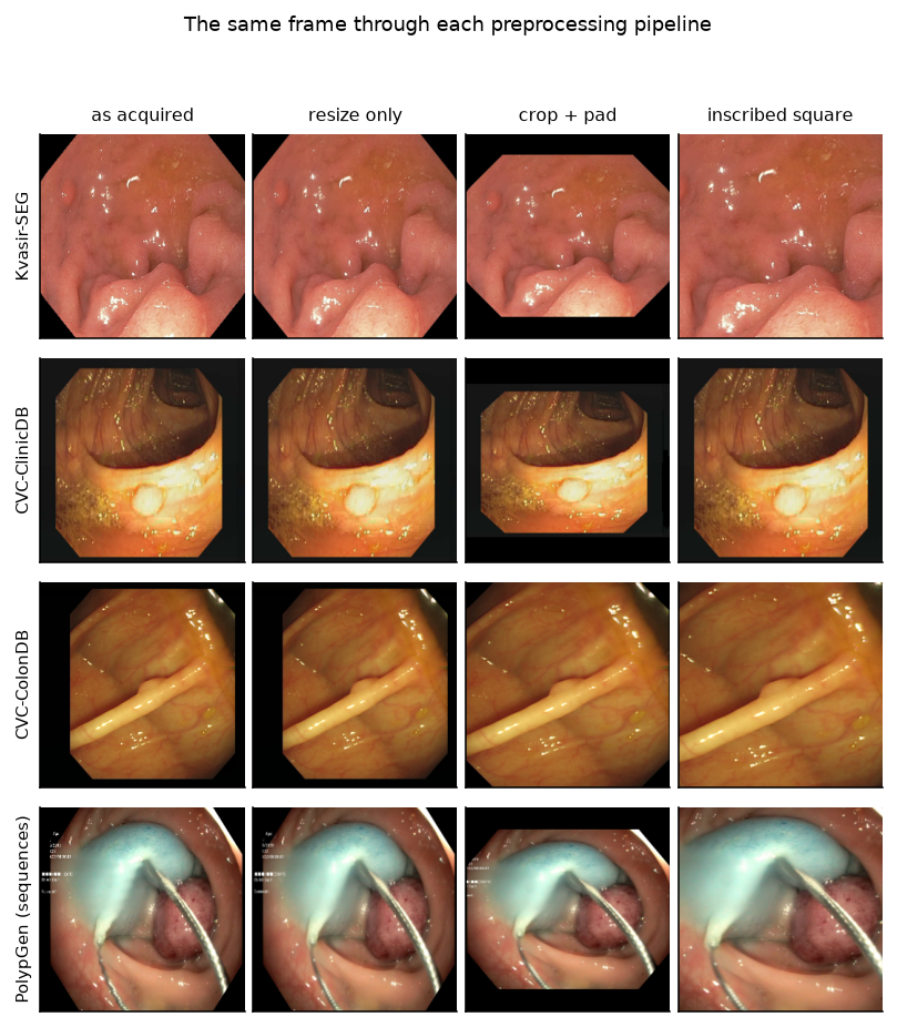
An endoscope hands you tissue inside a frame the equipment drew: black letterboxing, an octagonal field-of-view mask, the exam date burned into the pixels, the processor's settings. None of it is anatomy. All of it identifies the machine — and the machine correlates with the answer. Five public colonoscopy datasets, three centres.
1 · A frame announces where it came from
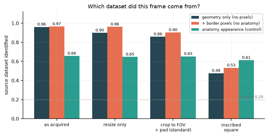
Nine descriptors of the canvas geometry — aspect ratio, mask area fraction, letterbox extents, centroid offset — and no anatomy pixels at all. A classifier on those nine numbers picks the right dataset out of five:
| as acquired | 0.961 |
| resize only | 0.899 |
| crop to the field of view + pad — the standard recipe | 0.859 |
| inscribed square — geometry removed | 0.477 |
| chance | 0.200 |
The standard fix barely works. Cropping to the imaging area and padding to a square — what most pipelines do — moves it 0.90 to 0.86, because padding preserves the aspect ratio deliberately, so as not to distort anatomy, and carries the signature along with it.
2 · Self-supervision makes it structural
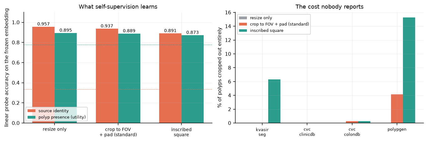
A contrastive loss pushes apart different images. If the source is identifiable, the cheapest way to push two images apart is to notice they came from different equipment — so the pretext task gets solved on the letterbox. And self-supervision exists in order to pool sources, so the exposure grows with the very thing that makes it worth doing.
A small encoder pretrained on pooled frames, frozen, then linearly probed:
| pipeline | source identity chance 0.33 | polyp presence chance 0.78 |
|---|---|---|
| resize only | 0.957 | 0.895 |
| crop to the field of view + pad | 0.937 | 0.889 |
| inscribed square | 0.891 | 0.873 |
The learned encoder recovers almost everything cropping removed: 0.86 to 0.48 for hand-made features, but only 0.96 to 0.89 here. It reads colour, illumination and texture — not border shape. Removing the geometry does not remove the confound, it moves it.
3 · The non-anatomical part predicts the diagnosis
HyperKvasir, restricted to the lower GI tract so that scope type cannot act as a confound:
| geometry only | 0.488 |
| border pixels — no anatomy | 0.674 |
| anatomy colour statistics | 0.666 |
| majority class | 0.172 |
The border region beats the anatomy's own colour statistics. What leaks is the session — dye, illumination settings, timestamp — and the session correlates with why the procedure was done in the first place. Upper against lower GI is 99.5% predictable from geometry alone.
4 · Removing the shortcut does not buy generalisation
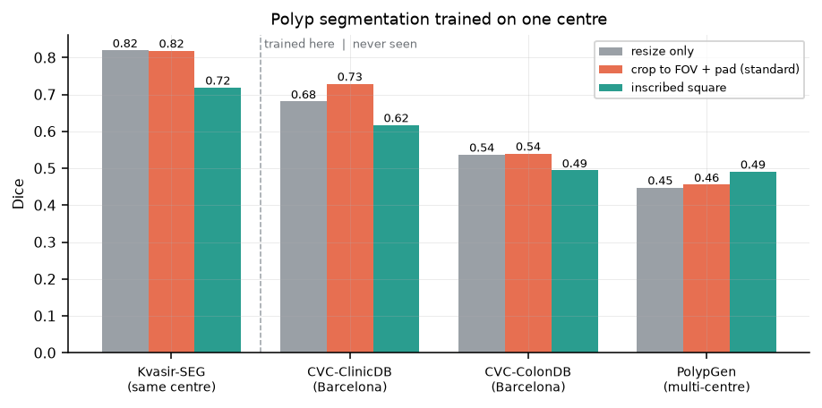
This is the part that did not work, and it is the most informative one. Polyp segmentation trained on the Norwegian data, Dice on frames that contain a polyp:
| pipeline | Kvasir same centre | CVC- ClinicDB | CVC- ColonDB | Polyp- Gen |
|---|---|---|---|---|
| resize only | 0.820 | 0.681 | 0.537 | 0.448 |
| crop + pad | 0.819 | 0.729 | 0.540 | 0.456 |
| inscribed square | 0.719 | 0.618 | 0.494 | 0.491 |
Crop-and-pad is free and mildly helpful. The inscribed square removes the most signature, loses 10 Dice in-distribution, and wins only on the most heterogeneous target.
Three explanations fit, and this experiment separates none of them. The model may never have used the shortcut. Losing 24% of the imaged area may simply cost more than the shortcut was worth. Or — found only afterwards — the crop removes the polyp entirely from 6.3% of Kvasir and 15.3% of PolypGen frames, so part of the training is on corrupted labels. The last explanation is the dullest and probably the largest.
A curation confound underneath all of it
| dataset | distinct resolutions | median coverage |
|---|---|---|
| Kvasir-SEG · Norway · n=1,000 | 98 | 0.825 |
| HyperKvasir · Norway · n=10,662 | 58 | 0.935 |
| CVC-ClinicDB · Barcelona · n=612 | 1 | 0.720 |
| CVC-ColonDB · Barcelona · n=380 | 1 | 0.837 |
| PolypGen · multi-centre · n=2,225 | 8 | 0.834 |
Kvasir keeps the native acquisition resolution; the CVC sets were normalised to exactly one before release. That is curation, not biology, and it is baked into every benchmark that trains on one and tests on the other.
What this does not show
That any published model took the shortcut — every result here is correlational. Three centres, not six. One training centre for the segmentation arm. The self-supervised encoder is small and trained from scratch, not a foundation model. No clinical claim of any kind.
Reproduce it
Everything runs from public data: five colonoscopy datasets, a single command per experiment, 29 tests in CI on Python 3.11–3.13. The negative result in section 4 is in the repository with the code that produced it.